An Analysis of Eminem Lyrics - NLP

Filtering out non-Eminem lyrics

Since we are doing an analysis on Eminem lyrics, we remove any lyrics performed by other artists. These are guest features performing intros, outros, choruses, hooks, or verses. This process is made easy since the lyrics data returned by the geniusr package also includes a section_name and section_artist variable. These are based on how Genius labels song sections. Importantly, the section_artist for the song Arose is wrong, so we have to handle it separately from the other songs. The code for this process is shown below:

# Filter out lines whose section artists do not include Eminem
lyrics<-original_lyrics %>%
  filter(str_detect(section_artist, "Eminem")|
         section_artist=="Arose"|
         section_artist=="Castle Extended") %>%
  rename(lyric=line, track_n=track_number) %>%
  group_by(song_name) %>%
  mutate(line=cumsum(song_name==song_name)) %>%
  select(lyric, line, album, track_n, song_name, album_year) %>%
  ungroup()

Fixing contractions

Contractions are commonplace in lyrics, so we have to expand as many as we can find. I define a function fix_contractions that replaces various contractions with their expanded forms. These include common contractions in English as well as some special ones I found after exploring the data.

# first change to lowercase to for consistency
lyrics$lyric<-tolower(lyrics$lyric)

# this is a function to fix contractions. These are contractions I identified
# after exploring the data for some time.
fix_contractions<-function(dat){
  # as in the article, this could be a possesive or is/has
  dat<-str_replace_all(dat, "'s", "")
  dat<-str_replace_all(dat, "'m", " am")
  # this one could be had or would, but I decide to replace with would
  # barring analysis of tense, which I don't intend to do, this probably has no effect
  dat<-str_replace_all(dat, "'d", " would")
  # special cases of the n't contraction - won't and can't
  dat<-str_replace_all(dat, "can't", "cannot")
  dat<-str_replace_all(dat, "won't", "will not")
  dat<-str_replace_all(dat, "don'tchu", "don't you")
  # ain't is a special case.
  dat<-str_replace_all(dat, "ain't", "aint")
  dat<-str_replace_all(dat, "n't", " not")
  dat<-str_replace_all(dat, "'re", " are")
  dat<-str_replace_all(dat, "'ve", " have")
  dat<-str_replace_all(dat, "'ll", " will")
  dat<-str_replace_all(dat, "y'all", "you all")
  dat<-str_replace_all(dat, "e'ry", "every")
  dat<-str_replace_all(dat, "'da", " would have")
  dat<-str_replace_all(dat, "a'ight", "all right")
  dat<-str_replace_all(dat, "prob'ly", "probably")
  dat<-str_replace_all(dat, "'em", "them")
  # gerund contractions
  dat<-str_replace_all(dat, "in'\\s", "ing  ")
  # finna, wanna, gonna
  dat<-str_replace_all(dat, "gonna", "going to")
  dat<-str_replace_all(dat, "finna", "going to")
  dat<-str_replace_all(dat, "wanna", "want to")
  dat
}
lyrics$lyric<-fix_contractions(lyrics$lyric)

Removing alphanumeric characters

Here we want to make sure that we drop any punctuation marks or any other special characters. For this analysis, we want to focus on only text.

# remove alphanumeric characters
lyrics$lyric <- str_replace_all(lyrics$lyric, "[^a-zA-Z0-9 ]", " ")

Filtering out any skits/intros/interludes.

Here we filter out any shorter Eminem verses, which turn out to be mostly skits, intros, outros, and interludes.

# removeing skits, intros, outros, interludes
line_count<-lyrics %>%
  group_by(album, song_name) %>%
  count() %>%
  ungroup() %>%
  arrange(n)

short_titles<-subset(line_count, n<15)$song_name

lyrics<-lyrics%>%
  filter(!str_detect(song_name, "Skit"),
         !str_detect(song_name, "skit"),
         !song_name %in% short_titles)

Lemmatization

Lemmatization is the process of resolving words to their dictionary form. For example, any words in their gerund form (e.g. rapping) will be reduced to their dictionary form (rap). Skipping this process might affect the results of our analysis.

lyrics<-lyrics %>%
  mutate(lyric=textstem::lemmatize_strings(lyric))
lyrics

## # A tibble: 14,455 x 6
##    lyric                   line album          track_n song_name      album_year
##    <chr>                  <int> <chr>            <dbl> <chr>          <date>    
##  1 yes                        1 Music To Be M~       1 Premonition (~ 2020-01-17
##  2 so i guess this be wh~     2 Music To Be M~       1 Premonition (~ 2020-01-17
##  3 think it obvious           3 Music To Be M~       1 Premonition (~ 2020-01-17
##  4 we aint never go to s~     4 Music To Be M~       1 Premonition (~ 2020-01-17
##  5 but it funny               5 Music To Be M~       1 Premonition (~ 2020-01-17
##  6 as much as i hate you      6 Music To Be M~       1 Premonition (~ 2020-01-17
##  7 i need you                 7 Music To Be M~       1 Premonition (~ 2020-01-17
##  8 this be music to be m~     8 Music To Be M~       1 Premonition (~ 2020-01-17
##  9 they say my last albu~     9 Music To Be M~       1 Premonition (~ 2020-01-17
## 10 no i sound like a spi~    10 Music To Be M~       1 Premonition (~ 2020-01-17
## # ... with 14,445 more rows

Word Frequencies

Depending on the analysis, there might be additional cleaning steps we might want to take. We often find that words such as a, an, the, and I, among others, are common across many documents in natural language data and are used with very high frequency. These are called stop words and they offer little insight into describing or classifying documents; therefore, they often removed prior to certain types of analysis. In the case of analyzing word frequencies, we want to remove stop words from our data set. The tidytext (Silge and Robinson 2016) package offers a set of stop words that we can import and use. First, we use unnest_tokens to convert our data frame to tidy text format; recall that the original data set had each line occupying a row. This function converts this so that each word occupies its on row. Next we remove stop words using an anti_join operation. The code is as below:

data("stop_words")

lyrics_filtered<-lyrics %>%
  unnest_tokens(word, lyric) %>%
  anti_join(stop_words) %>%
  ungroup()

words_total<-lyrics_filtered %>%
  count(word) %>%
  arrange(-n)

words_total

## # A tibble: 7,529 x 2
##    word      n
##    <chr> <int>
##  1 fuck    819
##  2 shit    509
##  3 aint    405
##  4 time    343
##  5 bitch   329
##  6 feel    324
##  7 love    263
##  8 leave   212
##  9 shady   190
## 10 girl    181
## # ... with 7,519 more rows

To no one’s surprise, Eminem curses a lot. His most used words are fuck and shit, and at number 4 we have bitch as well. This might generate interesting insights in case we compare it to other rappers. But on its own, I doubt its usefulness. There are other ‘non-useful words’ that I have identified through manual exploration of the data set. Throughout any analysis, you will have to deal with uncertainty and make micro decisions like this along the way. It is possible that removing these words will affect other parts of the analysis significantly. For now, we remove these words.

unnecessary_words <- c("fuck", "ah", "yeah", "aint", "shit","ass", "la", 
                       "yah", "ah", "bitch", "ama", "ha", "yo", "ah", "cum",
                       "dick", "ho", "erra", "gotta", "tryna", "gon", "dum",
                       "uh", "hey", "whoa", "til", "chka", "ta", "tahh")

lyrics_filtered <- lyrics_filtered %>%
  filter(!word %in% unnecessary_words)

words_total<-lyrics_filtered %>%
  count(word) %>%
  arrange(-n)

words_total

## # A tibble: 7,503 x 2
##    word      n
##    <chr> <int>
##  1 time    343
##  2 feel    324
##  3 love    263
##  4 leave   212
##  5 shady   190
##  6 girl    181
##  7 day     173
##  8 call    170
##  9 baby    168
## 10 world   158
## # ... with 7,493 more rows

Eminem uses the words love and feel frequently, so we get the idea that some major topics in Eminem’s songs are about love, emotions, and maybe relationships. Eminem has had many songs about relationships, although in most of them he portrays himself as being involved in a somewhat dysfunctional relationship. (See Love The Way You Lie and Good Guy). Eminem also uses shady frequently, so he is more likely to talks about his supposedly evil and unhinged alter-ego, Slim Shady.
We might be interested in the differences in word frequency across albums. Here we want to look at proportions, since absolute frequencies can lead to misleading conclusions.

freq<-lyrics_filtered %>%
  count(album, word) %>%
  group_by(album) %>%
  mutate(total=sum(n)) %>%
  mutate(freq=n/total) %>%
  ungroup() %>%
  arrange(-freq)

top10_freq<-freq %>%
  group_by(album) %>%
  top_n(8, freq) %>%
  ungroup() %>%
  arrange(album, freq) %>%
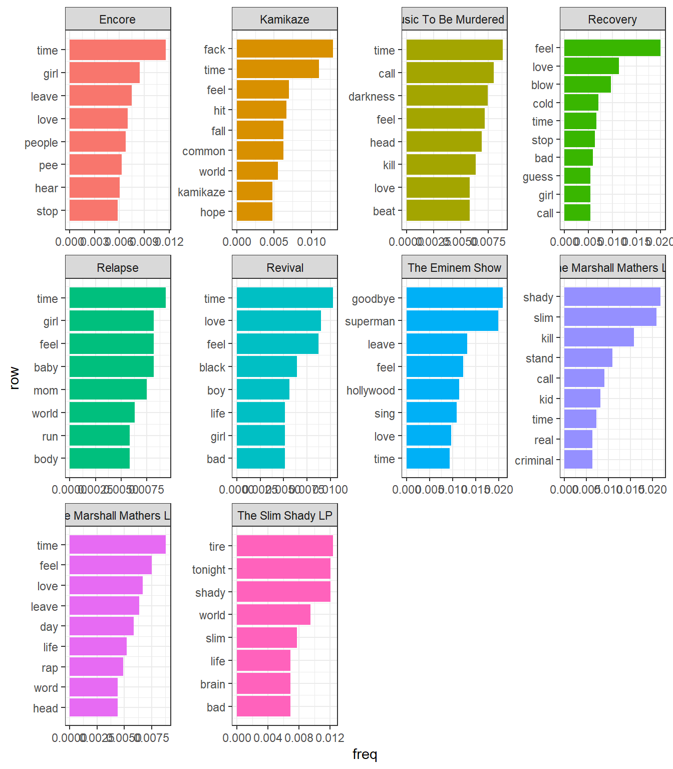
  mutate(row = row_number())

top10_freq %>%
  ggplot(aes(row, freq, fill=album)) +
  geom_col(show.legend = FALSE) +
  facet_wrap(~album, ncol=3, scales="free") +
  scale_x_continuous(breaks=top10_freq$row, 
                     labels=top10_freq$word) + 
  coord_flip() +
  theme_bw()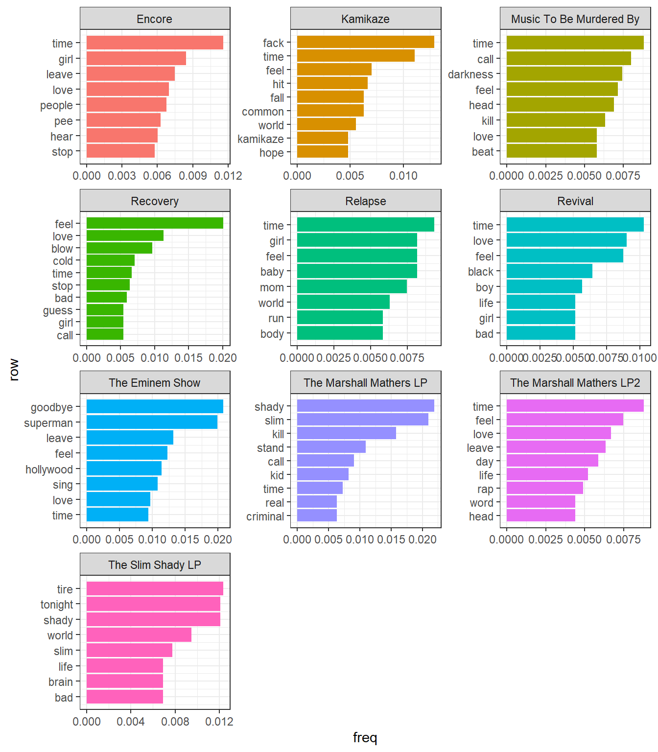

Here are some things we can note from this graph:

• Many of the frequently occurring words in these albums are simply those repeated in hooks and choruses. For example, in the album Recovery, we have cold and blow, which most likely comes from the song Cold Wind Blows. In the album The Eminem Show, we have goodbye, hollywood from Say Goodbye Hollywood and superman from, well, Superman.
• Time is a re-occuring theme. At this moment, however, I cannot say anything definitive about its significance.
  
• His first 2 albums feature a lot of use of slim and shady, which makes sense as this was when he introduced himself and his alter-ego to the world. It could also be as a result of the words being repeated in choruses some songs in the albums.
• Notice the lack of Hailie, his daughter, or Kim, his wife. One of the major reoccuring themes in Eminem’s music has been his love for his daughter and his hate for his wife. Contrary to my expectations, these words do not appear among the most frequently used words.
• Another major theme which lacks representation in the above graph is drugs. A probable reason for this is that Eminem namedrops many different drugs across his discography, which means that the word count for this theme is distributed across many different words.

words_total %>%
  filter(word %in% c("hailie", "kim"))

## # A tibble: 2 x 2
##   word       n
##   <chr>  <int>
## 1 hailie    37
## 2 kim       26

drugs<-c("Ambie", "Amoxicilline", "Coke", "Crack", "Codeïne", "Hydrocodone",
         "Klonopin", "Lean", "LSD", "Methadone", "Marijuana", "Mollie",
         "Mushrooms", "NoDoz", "Nurofen", "NyQuil", "Percocets", "Purple Haze",
         "Seroquel", "Smack", "Valium", "Vicodin", "Xanax", "Methamphetamine")
drugs<-str_to_lower(drugs)

words_total %>% 
  filter(word %in% c(drugs, "pill", "drug")) %>%
  count(wt=n)

## # A tibble: 1 x 1
##       n
##   <int>
## 1   217

Zipf’s law

In simple terms, this law states that given a list of terms from an arbitrary document/book, the frequency of each word is inversely proportional to its rank (rank measured in frequency). That implies that rank 1, the most used word, is used roughly twice as much as the rank 2 word, and 4 times as much as the rank 3 word, et cetera. See this Wikipedia post and Chapter 3 of Tidy Text Mining for a more in-depth explanation of this law. We can explore this concept with our word count data as well. First, let’s check the distribution of words in our data set. In this case, we stick to the unfiltered lyrics (lyrics with stop_words and unnecessary_words present).

unfiltered_total<-lyrics %>%
  ungroup() %>% # previously grouped
  unnest_tokens(word, lyric) %>%
  count(word, sort=TRUE)
  
unfiltered_total %>%
  ggplot(aes(x=n)) +
  geom_histogram(bins=40, color="black", fill="lightblue")+
  geom_hline(yintercept=0)+
  theme_bw() + xlab("total word count") + ylab("frequency of word count") +
  xlim(0, 50)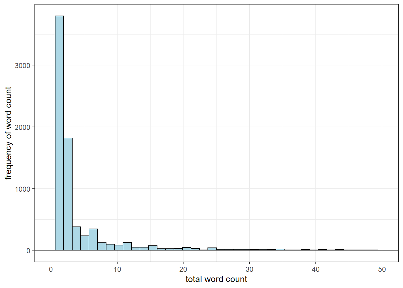

This distribution is known as the zeta distribution and comes about as a result of Zipf’s law, but it’s applications extend beyond modeling the relationship between the rank-frequency of words in natural language.
To the left of the distribution, we have a few popular words that are used most frequently by Eminem. The long right tail of the distribution in turn shows that there are many words that are used much less frequently.
A way to test whether a natural language dataset conforms to Zipf’s law is to plot a rank-frequency graph, on a log-log scale. In this case, the plotted line should have a negative slope and a linear relationship. In this case, I want to see if different albums conform to zipfs law

albums_total<-lyrics %>%
  unnest_tokens(word, lyric) %>%
  count(album, word, sort=T) %>%
  group_by(album) %>%
  mutate(total = sum(n))

albums_total

## # A tibble: 20,414 x 4
## # Groups:   album [10]
##    album                    word      n total
##    <chr>                    <chr> <int> <int>
##  1 The Marshall Mathers LP2 i      1075 19918
##  2 Recovery                 i       901 15649
##  3 The Marshall Mathers LP2 be      877 19918
##  4 The Marshall Mathers LP  i       778 11996
##  5 Music To Be Murdered By  i       714 11888
##  6 Revival                  i       705 13244
##  7 Relapse                  i       684 14669
##  8 Encore                   i       678 15173
##  9 Recovery                 you     672 15649
## 10 The Marshall Mathers LP2 the     652 19918
## # ... with 20,404 more rows

# we get frequency by rank
freq_by_rank <- albums_total %>%
  group_by(album) %>%
  mutate(rank = row_number(),
         `term frequency` = n/total)

# plot rank-frequency
freq_by_rank %>%
  ggplot(aes(rank, `term frequency`, color=album))+
  geom_line(size=1.1, alpha=0.8, show.legend=FALSE)+
  scale_x_log10() +
  scale_y_log10() +
  theme_bw()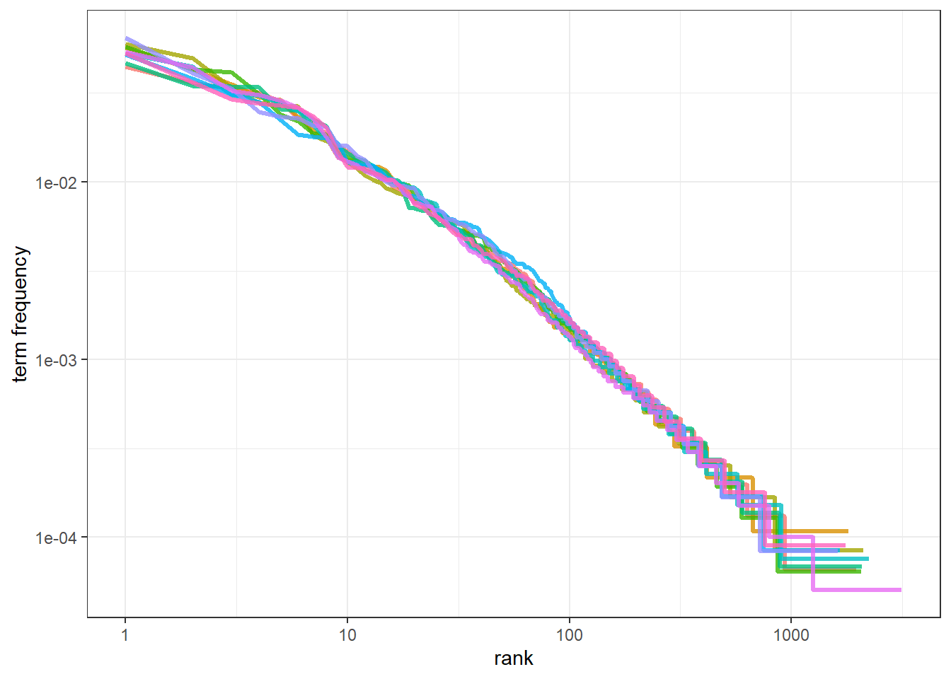

Intuitively, Zipf’s law suggests that the frequency of a word decreases rapidly with rank. We see that in this plot as well. The lines have slight curve and show greater deviation towards the its extremes; the relationship is thus not perfectly linear. Regardless, we can see the inverse relationship between the rank of a term and its frequency.

Word length

Hip hop music places emphasis on a rapper’s ability to rhyme. In addition, there is also the basic requirement that the artist should rap on beat. However, Eminem is known to easily pull off multi-syllabic rhymes. The image below shows a section of his song Stay Wide Awake where the words he’s rhyming are highlighted.

Furthermore, he is also able to rap fast, which means he can fit more words into a line and still remain on beat. Therefore, even though longer words are probably harder to rhyme and fit into a line, Eminem is theoretically able to overcome this limitation with ease. In any case, words lengths are an interesting measure to explore.

word_lengths<-lyrics %>%
  unnest_tokens(word, lyric) %>%
  select(song_name, album, word) %>%
  group_by(song_name, album) %>%
  distinct() %>%
  mutate(word_length=nchar(word)) %>%
  ungroup() %>%
  arrange(-word_length)
# summary(word_lengths)

# plot it
word_lengths %>%
  count(word_length, sort=TRUE) %>%
  ggplot(aes(x=word_length, y=n)) +
  geom_col(show.legend=F, fill="lightblue", 
           color="black") +
  xlab("word length") + ylab("word count") +
  ggtitle("word length distribution")+
  theme_bw()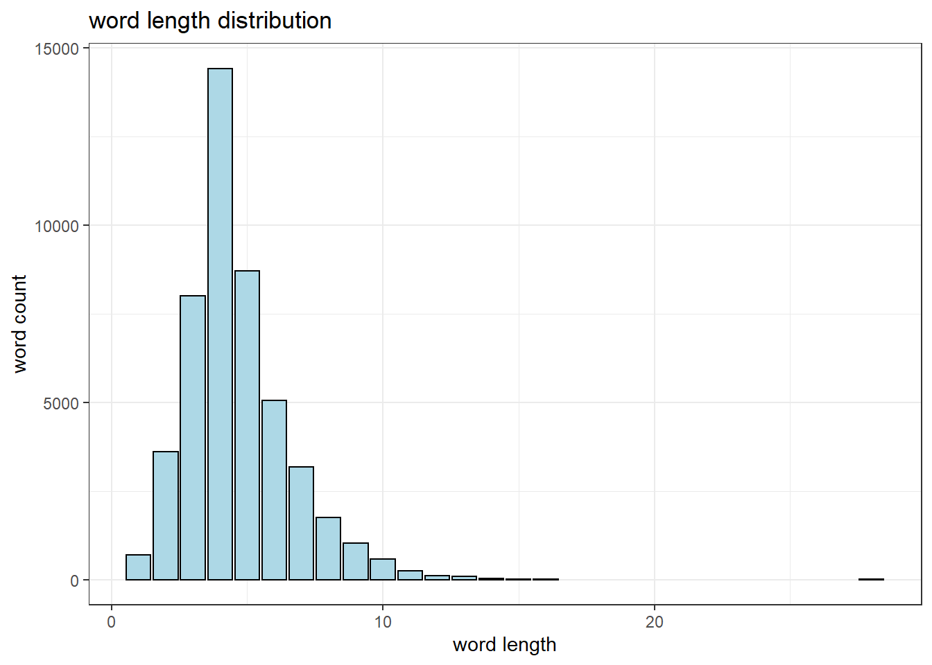

The most frequently used words are 3-5 letters long. The distribution has a slightly long right tail and an outlier which is the 28 letter word, antidisestablishmentarianism. This analysis would probably be more interesting if we compare Eminem to other artists.
We can create word clouds based on length to visualize the word lengths.

# wordlength word cloud
wl_wc<-word_lengths %>%
  ungroup() %>%
  select(word, word_length) %>%
  distinct() %>%
  arrange(-word_length)

wordcloud2(wl_wc[1:300,],
           size=.15, minSize=.0005,
           ellipticity=0.3, rotateRatio=1,
           fontWeight="bold")

Lexical diversity and density

An article, attempted to determine which rapper has the largest vocabulary by counting the number of unique words in the first 35,000 by different artists. I extend this analysis by looking at the number of unique words used by Eminem across his 10 albums (lexical diversity). I also look at the number of unique words divided by the total number of words for each album (lexical density).

lyrics %>%
  unnest_tokens(word, lyric) %>%
  summarise(unique=n_distinct(word))

## # A tibble: 1 x 1
##   unique
##    <int>
## 1   7915

We got 7884 unique words. Remember that our data set only includes lyrics from his studio albums. Let’s analyze lexical diversity across his albums.

lexical_diversity_per_album<-lyrics %>%
  unnest_tokens(word, lyric) %>%
  group_by(song_name, album, album_year) %>%
  summarize(lex_diversity=n_distinct(word)) %>%
  # mutate(album=reorder(album, album_year)) %>%
  arrange(-lex_diversity) %>%
  ungroup()

# lex diversity plot
lexical_diversity_per_album %>%
  ggplot(aes(album_year, lex_diversity)) +
  geom_point(color="red", size=4, alpha=.4) +
  stat_smooth(color="black", se=TRUE, method="lm") +
  geom_smooth(aes(x=album_year, y=lex_diversity), se=FALSE, color="blue", lwd=2) +
  ggtitle("Lexical diversity") +
  ylab("") + xlab("") +
  theme_bw()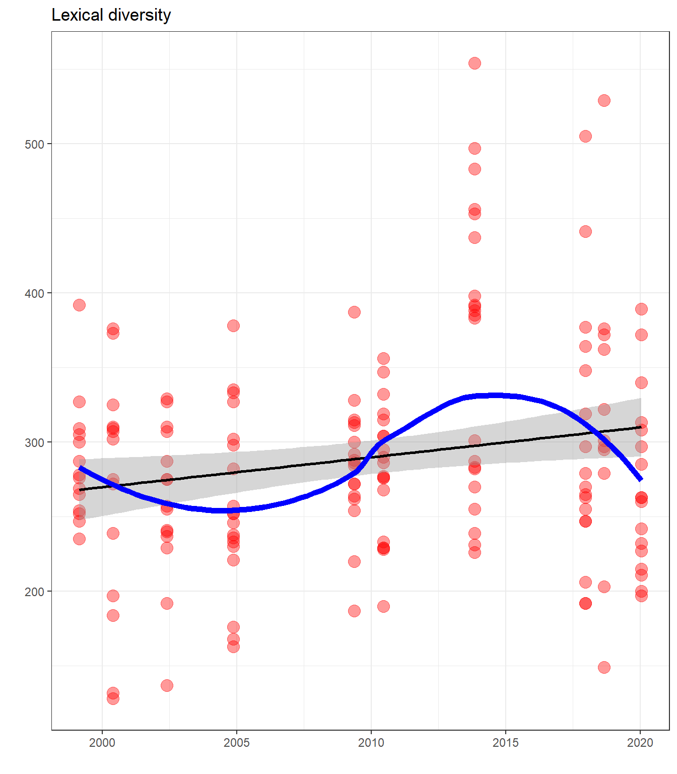

There’s a slight increase in lexical diversity across album time. Surprisingly, his latest album, Music To Be Murdered By, has a lower lexical diversity than his previous two. MMLP2, Kamikaze, and Revival have the highest lexical diversities.

To contrast, we can also explore lexical density.

## LEXICAL DENSITY
lexical_density_per_album <- lyrics %>%
  unnest_tokens(word, lyric) %>%
  group_by(song_name, album, album_year) %>%
  summarize(lex_density=n_distinct(word)/n()) %>%
  arrange(-lex_density) %>%
  ungroup()

lexical_density_per_album

## # A tibble: 164 x 4
##    song_name            album                   album_year lex_density
##    <chr>                <chr>                   <date>           <dbl>
##  1 Session One          Recovery                2010-06-18       0.585
##  2 When the Music Stops The Eminem Show         2002-05-26       0.548
##  3 Yah Yah              Music To Be Murdered By 2020-01-17       0.538
##  4 Remember Me?         The Marshall Mathers LP 2000-05-23       0.528
##  5 Good Guy             Kamikaze                2018-08-31       0.527
##  6 Nice Guy             Kamikaze                2018-08-31       0.503
##  7 Bad Meets Evil       The Slim Shady LP       1999-02-23       0.490
##  8 Bitch Please II      The Marshall Mathers LP 2000-05-23       0.482
##  9 You Gon’ Learn       Music To Be Murdered By 2020-01-17       0.481
## 10 Lock It Up           Music To Be Murdered By 2020-01-17       0.477
## # ... with 154 more rows

# plot 
lexical_density_per_album %>%
  ggplot(aes(album_year, lex_density)) +
  geom_point(color="green", alpha=0.4, size=4, position="jitter") +
  stat_smooth(color="black", se=FALSE, method="lm") +
  geom_smooth(se=FALSE, color="blue", lwd=2) +
  ggtitle("Lexical density") + xlab("") + ylab("") +
  theme_bw()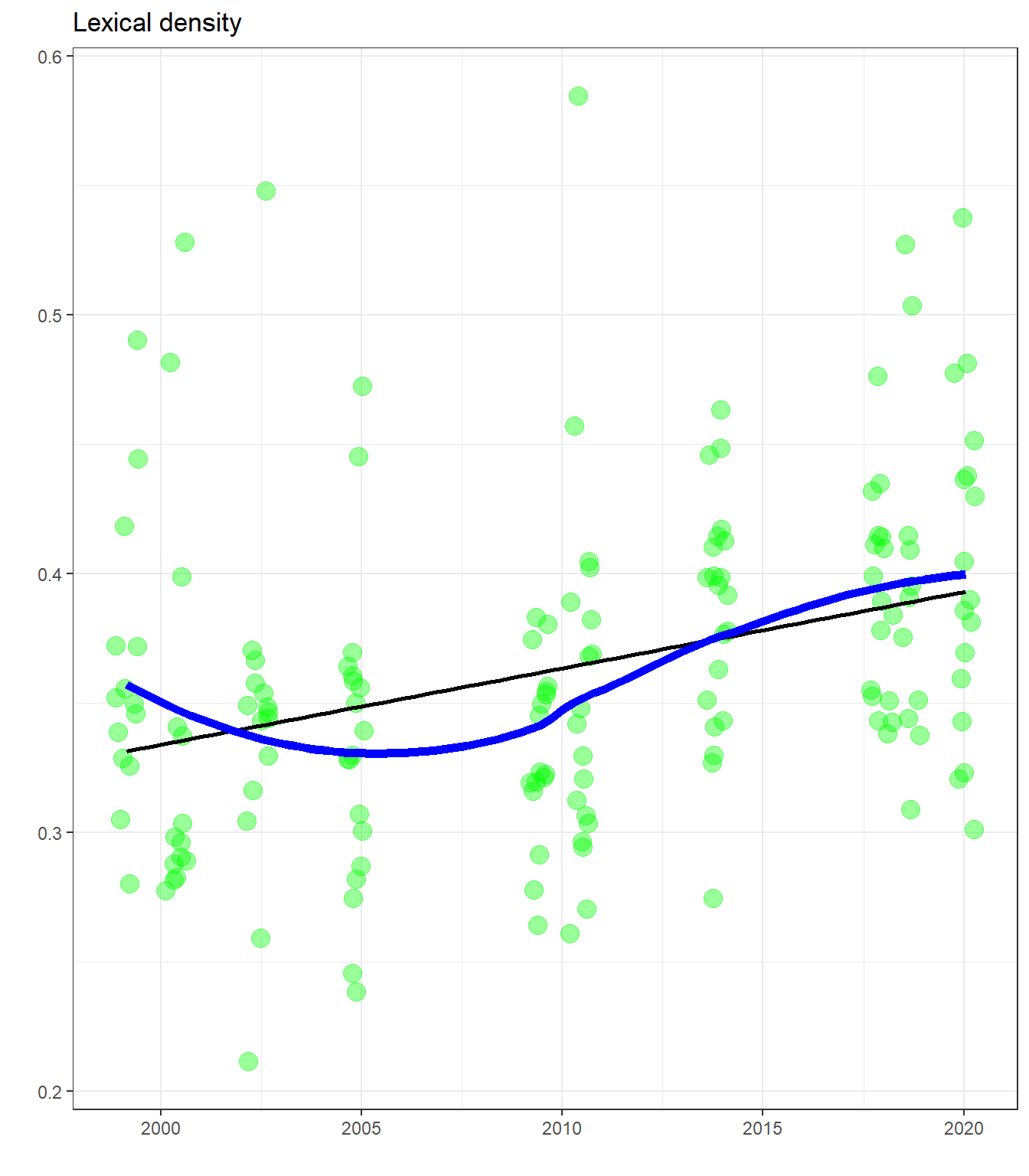

Here we see an increase in lexical density over time, indicating a decrease in repetition with each new album he puts out.

tf-idf

Here we use tidytext’s bind_tf_idf function in a neat way to find the tf-idf for each of these words - tf-idf is a measure of how important a word is to a particular document. If a word is used frequently across all albums, then it’s not indicative of or significant to any particular album. But if a word is used in only one album relatively frequently, then we can think of this word as of significance to that album.

lyrics_tf_idf <- lyrics %>%
  unnest_tokens(word, lyric) %>%
  distinct() %>%
  count(album, word, sort=TRUE) %>%
  ungroup() %>%
  bind_tf_idf(word, album, n) %>%
  arrange(-tf_idf)

# plot the top tf-idf
top_tf_idf <- lyrics_tf_idf %>%
  arrange(-tf_idf) %>%
  mutate(word = factor(word, levels = rev(unique(word)))) %>%
  group_by(album) %>%
  slice(seq_len(8)) %>%
  ungroup() %>%
  arrange(album, tf_idf) %>%
  mutate(row=row_number())

top_tf_idf %>%
  ggplot(aes(x=row, y=tf_idf, fill=album)) +
  geom_col(show.legend=FALSE) +
  labs(x=NULL, y="TF-IDF") +
  ggtitle("Most important words using tf-idf by album") +
  theme_bw() +
  facet_wrap(~album, scales="free", ncol=3) +
  scale_x_continuous(breaks=top_tf_idf$row,
                     labels=top_tf_idf$word) +
  coord_flip()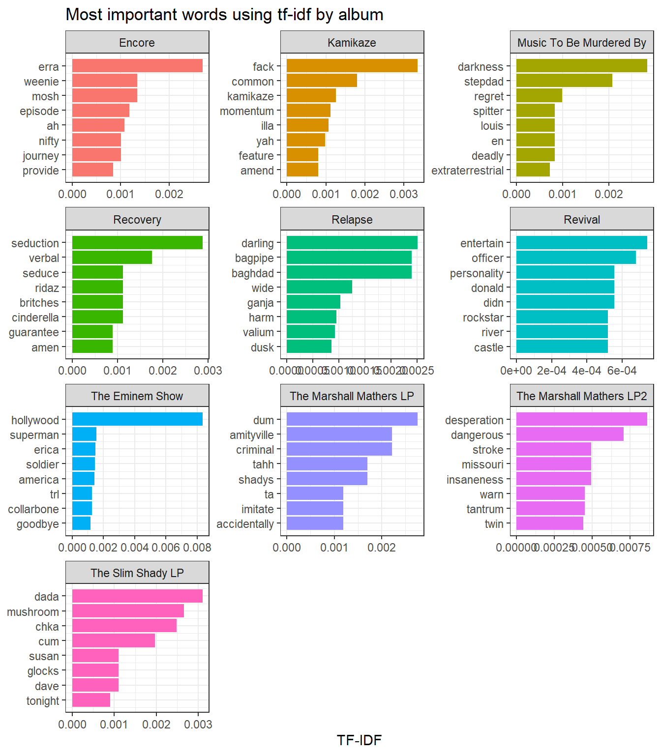

We can get some insights if we compare this to the word frequency plot we did earlier; I have placed it here again for ease of comparison. Recall that in that plot, the words feel, time, and love appeared frequently in almost all of the albums. Therefore, these words cannot be used to distinguish between albums. On the other hand, the words goodbye, hollywood, and superman which we saw corresponded to specific songs also have appear in the set of words with the highest tf-idf’s. These terms are indicative of particular songs, which then helps distinguish albums from each other. Many of the top tf-idf terms correspond to song titles that are also repeated in choruses and hooks. To some extent, we can get a sense of the topics of songs included in each particular album.

References

Dantas, Tiago Mendes. 2018. Rspotify: Access to Spotify Api. https://CRAN.R-project.org/package=Rspotify.
Henderson, Ewen. 2020. Geniusr: Tools for Working with the ’Genius’ Api. https://CRAN.R-project.org/package=geniusr.
Silge, Julia, and David Robinson. 2016. “Tidytext: Text Mining and Analysis Using Tidy Data Principles in R.” JOSS 1 (3). https://doi.org/10.21105/joss.00037.
Wickham, Hadley. 2016. Ggplot2: Elegant Graphics for Data Analysis. Springer-Verlag New York. https://ggplot2.tidyverse.org.
Wickham, Hadley, Romain François, Lionel Henry, and Kirill Müller. 2020. Dplyr: A Grammar of Data Manipulation. https://CRAN.R-project.org/package=dplyr.